Vector Field
RenderableVectorField renders a 3D vector field as a collection of arrows. Each arrow represents the direction and magnitude of a vector at a specific point in space. This page describes how to load a vector field dataset and the options for controlling the appearance of the vector arrows.
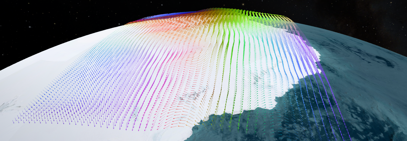
An example of a vector field rendered in OpenSpace using the sparse mode with direction-based coloring.
Loading Vector Field Datasets
There are two ways to load vector field data into OpenSpace. The renderable supports two input modes: a regular volumetric grid and a sparse point-cloud dataset. Both modes provide several options for coloring, scaling, and filtering the result.
The Mode parameter controls how the vector field data is loaded and interpreted. There are two options: Volume and Sparse.
Volume Mode
In Volume mode, the data is a regular 3D grid of velocity vectors stored in a raw binary file. The grid is mapped to a spatial domain defined by MinDomain and MaxDomain. Each voxel stores three floating-point values - the x, y, and z components of the velocity vector, packed tightly and written in little-endian format.
The voxel order is x-y-z meaning x is the innermost loop, followed by y, and z is the outermost. The example Python script below shows how to write the binary data:
import struct

# Volume dimensions
Nx = 32
Ny = 32
Nz = 32

with open("vectorfield.bin", "wb") as f:
  for z in range(Nz):
    for y in range(Ny):
      for x in range(Nx):
        f.write(struct.pack("<fff", vx, vy, vz))
A minimal asset using volume mode looks like the following:
...
Renderable = {
  Type = "RenderableVectorField",
  Mode = "Volume",
  Volume = {
    VolumeFile = asset.resource("data/vectorfield.bin"),
    -- Spatial extent of the volume, in meters
    MinDomain = { -1E8, -1E8, -1E8 },
    MaxDomain = {  1E8,  1E8,  1E8 },
    -- Number of voxels along each axis
    Dimensions = { 32, 32, 32 }
  }
}
...
Note
The Dimensions value must exactly match the grid size used when writing the binary file.
Sparse Mode
In Sparse mode, the data is a CSV file where each row corresponds to one vector. Each row must include three position columns and three velocity columns. By default the column names x, y, z (position) and vx, vy, vz (velocity) are assumed, but these can be overridden in the asset.
An example CSV file:
x,y,z,vx,vy,vz
13428000,26239000,45870000,-377.27,-161.05,282.85
10993567,30395576,-33872508,-2.15,217.11,-176.28
24999000,28370000,19911000,205.61,54.21,-261.05
Additional columns may be present in the file and will simply be ignored. A minimal asset using sparse mode looks like the following:
...
Renderable = {
  Type = "RenderableVectorField",
  Mode = "Sparse",
  Sparse = {
    FilePath = asset.resource("data/vectors.csv")
  }
}
...
If the CSV file uses different column names, specify them explicitly in the Sparse table:
...
Renderable = {
  Type = "RenderableVectorField",
  Mode = "Sparse",
  Sparse = {
    FilePath = asset.resource("data/vectors.csv"),
    X = "pos_x",
    Y = "pos_y",
    Z = "pos_z",
    Vx = "vel_x",
    Vy = "vel_y",
    Vz = "vel_z"
  }
}
...
Coloring
The vector field can be colored using three different color modes. These are set by adding a Coloring component to the Renderable specification. The color mode is controlled via ColorMode:
Fixed (default) - all arrows are drawn with the same single color, specified by FixedColor as an RGBA value in the range [0, 1]:
Coloring = {
  ColorMode = "Fixed",
  FixedColor = { 1.0, 0.5, 0.0, 1.0 }  -- orange
}
Magnitude - arrows are colored by the magnitude (speed) of the vector, using a color map file. The color map is a 1D texture that maps normalized magnitude values to colors. See the color map page for details about supported color map formats. The magnitude range can be set manually or left to be computed automatically from the data:
Coloring = {
  ColorMode = "Magnitude",
  ColorMap = asset.resource("colormaps/viridis.png"),
  -- Optional: override the auto-detected magnitude range
  ColorMappingDataRange = { 0.0, 500.0 }
}
Direction - arrows are colored by the direction they point, following this convention: +X -> Red, -X -> Cyan, +Y -> Green, -Y -> Magenta, +Z -> Blue, -Z -> Yellow. This mode requires no additional settings and is useful for quickly identifying the dominant flow direction.
Coloring = {
  ColorMode = "Direction"
}
Putting it all together, a Coloring component added to a sparse vector field looks like this:
...
Renderable = {
  Type = "RenderableVectorField",
  Mode = "Sparse",
  Sparse = {
    FilePath = asset.resource("data/vectors.csv")
  },
  Coloring = {
    ColorMode = "Magnitude",
    ColorMap = asset.resource("colormaps/viridis.png"),
    -- Optional: override the auto-detected magnitude range
    ColorMappingDataRange = { 0.0, 500.0 }
  }
  ...
}
...
Appearance Settings
There are additional settings that control the appearance of the vector field. These properties can also be adjusted interactively in the GUI under the scene graph node’s properties panel at runtime.
Property |
Default |
Description |
|---|---|---|
|
|
Scales the arrow lengths using an exponential scale, ranging from meter scale (1) to approximately 3 Mpc scale (100). |
|
|
Width of the arrow lines in pixels. |
|
|
Render only every n-th vector. A stride of 1 renders all vectors, 2 renders every other vector, 3 renders every third, and so on. This is useful for reducing visual clutter in dense datasets. |
Lua Filtering
For advanced use cases, it is possible to filter which vectors are displayed by providing a custom Lua script. This is useful for, for example, only showing vectors above a certain speed threshold or within a specific spatial region.
To enable filtering, set FilterByLua = true and point Script to a .lua file. The script must define a function called filter that receives the position (x, y, z) and velocity (vx, vy, vz) of a vector and returns true to include it, or false to exclude it:
-- example_filter.lua
function filter(x, y, z, vx, vy, vz)
  local magnitude = math.sqrt(vx * vx + vy * vy + vz * vz)
  -- Only show vectors with a speed greater than 100
  return magnitude > 100.0
end
In the asset, enable filtering like this:
...
Renderable = {
  Type = "RenderableVectorField",
  Mode = "Sparse",
  Sparse = {
    FilePath = asset.resource("data/vectors.csv")
  },
  FilterByLua = true,
  Script = asset.resource("scripts/example_filter.lua")
}
...
Note
The filter script is reloaded automatically whenever the file changes on disk, so you can iterate on your filter function without restarting OpenSpace.
Warning
If FilterByLua is set to true but the Script path is missing or the file cannot be found, filtering will be silently disabled.
Full Asset Example
The following example shows a complete asset using sparse mode with magnitude coloring and a Lua filter:
local Node = {
  Identifier = "WindVectors",
  Renderable = {
    Type = "RenderableVectorField",
    Mode = "Sparse",
    Sparse = {
      FilePath = asset.resource("data/wind.csv"),
      Vx = "u", Vy = "v", Vz = "w"
    },
    VectorFieldScale = 20.0,
    LineWidth = 1.5,
    Stride = 2,
    Coloring = {
      ColorMode = "Magnitude",
      ColorMap = asset.resource("colormaps/plasma.png")
    },
    FilterByLua = true,
    Script = asset.resource("scripts/wind_filter.lua")
  },
  GUI = {
    Name = "Wind Vectors",
    Path = "/Atmosphere"
  }
}

asset.onInitialize(function()
  openspace.addSceneGraphNode(Node)
end)

asset.onDeinitialize(function()
  openspace.removeSceneGraphNode(Node)
end)